モンテカルロ法(Pythonでの処理高速化_2)
■前回の処理高速化の続き。
前回、Numpy, Numba, Sobolといったいくつかの方法を使って、モンテカルロ法で円周率近似を行うコードの高速化を検討した。今回、それらを組み合わせてどのくらいの大きさまでできそうか見てみたい。
高速化の検討の中で、画面の描写処理がボトルネックとなっていたので、結果表示は最後に一度のみ行い純粋に演算処理だけにした。
前回Sobolの準乱数が一番速かったので、それを使って1.2億回の試行から120憶回に増やしてどのくらいかかるか見た。すると途中で下記のエラーが出た。デフォルトでは、2^30 ≒ 10.7億 までしか生成できないよう。
ValueError: At most 2**30=1073741824 distinct points can be generated. 1073600001 points have been previously generated, then: n=1073600001+400000=1074000001. Consider increasing bits.
bit数を増やせとのことだったので、36 (2^36≒687億)にして実行すると、今度は途中で止まってしまいエラーにもならない。ただ進まないだけ。ChatGPTに聞くと、2^32≒43億までが上限とのこと(SciPy の Sobol 実装の内部カウンタ制限32bit)。リセットして使いまわすこともできるようだけど、別の乱数生成を使う(rng = np.random.default_rng())。
Chat GPTで高速のコードを生成してもらい、最終的に一番下のコードで実行。Numpy, Numbaなどを組み合わせたもの。600憶回を13、14分ぐらいでできた(次の結果)。
| 試行 | Numpyベクトル化(1.2億回、対照として) | 結果 | 高速化(600憶回) | 結果 |
| 1 | 3.08 s | 3.1415751000 | 775.14 s | 3.1415956020 |
| 2 | 3.91 s | 3.1415204667 | 812.29 s | 3.1416049004 |
| 3 | 4.03 s | 3.1415917000 | 830.40 s | 3.1415908337 |
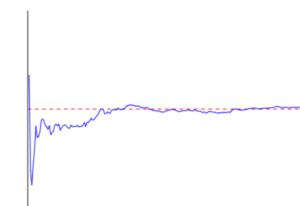
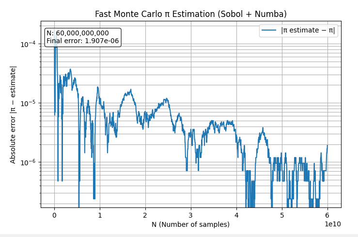
πへの近似は見た目では分からなくなってきたので、真値との差で対数表示とした。
πの真値(3.14159265358…)に近づくにつれ値が小さくなる。一番下がる傾向が出ているのが下だけど、必ずしも順調に下がる感じではない。
別の試行の結果。400憶ぐらいより先ではむしろ上がっている。
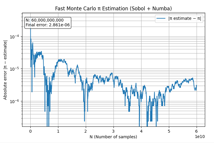
上のテーブルで実際に得られた結果でも、正しい値は4桁目(3.1415)または5桁目(3.14159)まで。処理時間とか考えると数時間あれば数千億ぐらいまではできそうだけど、これ以上の正しい値の桁を求めるのは難しいかもしれない。
■コードサンプル
import time
import math
import numpy as np
import matplotlib.pyplot as plt
from scipy.stats import qmc
from numba import njit, prange
N_MAX = 60_000_000_000 # 総サンプル数
STEP = 40_000_000 # 1バッチのサンプル数(大きいほど速い)
SAVE_POINTS = 3000 # 保存する履歴数
@njit(parallel=True, fastmath=True)
def count_inside(points):
cnt = 0
for i in prange(points.shape[0]):
x = points[i, 0]
y = points[i, 1]
if x * x + y * y <= 1.0:
cnt += 1
return cnt
inside_count = 0
total_count = 0
n_history = np.empty(SAVE_POINTS, dtype=np.int64)
pi_history = np.empty(SAVE_POINTS, dtype=np.float32)
save_interval = max(N_MAX // (STEP * SAVE_POINTS), 1)
save_index = 0
loop_counter = 0
sampler = qmc.Sobol(d=2, scramble=False, bits=36)
t_start = time.perf_counter()
rng = np.random.default_rng()
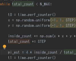
while total_count < N_MAX:
# Sobol 列生成
# points = sampler.random(STEP)
# points = np.random.random((STEP, 2))
points = np.empty((STEP, 2), dtype=np.float64)
rng.random(points.shape, out=points)
# inside 判定(Numba)
inside = count_inside(points)
inside_count += inside
total_count += STEP
loop_counter += 1
if loop_counter % save_interval == 0 and save_index < SAVE_POINTS:
pi_history[save_index] = 4.0 * inside_count / total_count
n_history[save_index] = total_count
save_index += 1
if (total_count / 100) % STEP == 0:
print(f"Progress (totalcount): {total_count:,}")
t_end = time.perf_counter()
mc_time_total = t_end - t_start
pi_history = pi_history[:save_index]
n_history = n_history[:save_index]
error_history = np.abs(pi_history - math.pi)
fig, ax = plt.subplots(figsize=(8, 5))
ax.plot(n_history, error_history, label="|π estimate − π|")
ax.set_yscale("log")
ax.set_xlabel("N (Number of samples)")
ax.set_ylabel("Absolute error |π − estimate|")
ax.set_title("Fast Monte Carlo π Estimation (Sobol + Numba)")
ax.grid(True, which="both")
ax.legend()
ax.text(
0.02, 0.95,
f"N: {total_count:,}\nFinal error: {error_history[-1]:.3e}",
transform=ax.transAxes,
fontsize=10,
verticalalignment="top",
bbox=dict(boxstyle="round", facecolor="white", alpha=0.8)
)
plt.show()
# ============================================================
# 結果表示
# ============================================================
print("==== Time summary ====")
print(f"Monte Carlo total time: {mc_time_total:.2f} s")
print(f"Total samples: {total_count:,}")
print(f"Final π estimate: {pi_history[-1]:.10f}")